Note
You can download this example as a Jupyter notebook or try it out directly in Google Colab.
6. Using advanced orders: Effects of regular block orders and linked orders#
This tutorial showcases the impact of regular block and linked orders in electricity market simulation outcomes.
In this example the advanced strategies using regular block orders and linked orders are presented and their impact on the market outcome both on system and unit level compared to strategies using only single hourly orders.
With the integration of block orders, minimum acceptance ratios are added to the orders as additional field. To account for those in the clearing, a new market clearing algorithm becomes necessary.
In this tutorial, we will show, how to create and integrate this advanced market clearing and adjust bidding strategies to allow the use of regular block orders and linked orders. Finally, we will create a small comparison study of the results using matplotlib.
As a whole, this tutorial covers the following
Explain the basic rules of block and linked orders.
Run a small example with single hourly orders.
Create the new market clearing algorithm.
Adjust a given strategy to integrate block orders.
Adjust a given strategy to integrate linked orders.
Extract graphs from the simulation run and interpret results.
1. Basics#
In general, most simulation studies only focus on single hourly orders. Yet, the reality includes a lot more than that, especially different types of block orders. The question is, how much do the advanced order types deviate the market outcome.
To showcase that ASSUME can handle different order types an advanced market clearing algorithm is created and tested with three different strategies. The testing scenarios are defined as 12 units (one for each technology) and an unflexible demand, cleared on a day-ahead market.
What are single hourly orders?
These are the simplest order structures implemented, also called simple orders. They can take the form of linear piece-wise curves containing interpolated orders only, step-wise curves containing step orders only, or a hybrid form of both. The general clearing of these orders strictly follows the merit order principle: any order with a bidding price below the MCP must be fully accepted, any order with a price above the MCP must be rejected, and orders where the price equals the MCP can be either accepted (fully/partially) or rejected.
What are block orders?
The characteristic of block orders is a time horizon that spans multiple minimum time units (MTUs). They are defined by a price, a number of time periods, some volumes that can be different for each period, and a constant minimum acceptance ratio (MAR). The MAR defines a restriction on how much a bid can be curtailed before it must be rejected. They can be divided into four subcategories:
Independent block orders (BOs): The elemental form is the regular block order, with constant volume and a MAR equal to 1, also referred to as “fill-or-kill”-condition. This determines that the volume must be entirely accepted or rejected. This BO-type is used most frequently and applied in all European power exchanges Devnath et al. 2020 and implemented in most models Tanrisever et al. 2020. Slight deviations are given with the curtailable BO, where the MAR can be below 1, and the profile BO, which includes volume changes over the block order periods.
Linked groups or linked orders (LOs): These groups of orders include parent and dependent child orders with the additional condition that the acceptance ratio of a parent order must be greater or equal to those of all child orders. During market clearing, children are considered, if they increase the profit. Hence, they can “save” the parent order, but not vice versa. There can be several levels of LOs in one group, but the number of children and levels is constrained by the power exchanges.
Exclusive groups: For this order type, the sum of acceptance ratios of a set of block orders must be below 1. If the MAR is set to 1, this results in an exclusive-or-relation of all orders in that group.
Flexible orders: These order structures are created through the formation of an exclusive group where the MAR is set to 1 and each order is shifted by one hour, introducing flexibility through the dispatch time determined by the algorithm, not predefined by the participant.
In this tutorial, we will compare the simple hourly orders with regular block orders and linked orders.
Bid formulation in this example
According to flexABLE, the inflexible and flexible power of a unit is bid seperately, compare Qussous et al. 2022.
The inflexible power \(P^{\mathrm{inflex}}_{t}\) at time \(t\) is the minimum volume that can by dispatched. It is defined by the current operation status of the unit, ramp-down limitations and the must-run time. The inflexible bid price depends on the marginal cost \(C^{\mathrm{marginal}}_t\) at time \(t\) and the power dispatch of the previous time step \(P^{\mathrm{dispatch}}_{t-1}\) and adds a markup, if the unit has to be started newly and a reduction, to prevent a shut-down, including the start-up costs \(C^{\mathrm{su}}_t\). Here, the average time of continuous operation is given by \(T^{\mathrm{op, avg}}\) and the average time of continuous shut down is given by \(T^{\mathrm{down, avg}}\): \begin{align} C^{\mathrm{inflex}}_t=C^{\mathrm{marginal}}_t + \frac{C^{\mathrm{su}}_t}{P^{\mathrm{inflex}}_{t} T^{\mathrm{op/down}}} \quad \mathrm{with} \: T^{\mathrm{op/down}} = \begin{cases} -T^{\mathrm{down, avg}}, & \mathrm{if} \: P^{\mathrm{dispatch}}_{t-1} > 0 \\ T^{\mathrm{op, avg}}, & \mathrm{otherwise} \end{cases} \end{align}
The flexible power \(P^{\mathrm{flex}}_{t}\) at time \(t\) is then the difference between maximum dispatchable volume and the inflexible power. It is defined by current operation status of the unit, ramp-up limitations and the must-operation time. The flexible bidding price is given by the marginal costs only:
\(C^{\mathrm{flex}}_t=C^{\mathrm{marginal}}_t\)
When transforming those bids into block orders, the volumes of the inflexible bids build the profile of one block bid over 24 hours. Because block orders are cleared according to the average market clearing price over the order period \(\mathcal{T}\), the price of the block order is given by the weighted average of the inflexible bid price:
\(C^{\mathrm{block}} = \frac{\sum_{t \in \mathcal{T}} C^{\mathrm{inflex}}_t \: P^{\mathrm{inflex}}_t}{\sum_{t \in \mathcal{T}} P^{\mathrm{inflex}}_t}\)
The linked orders are built by the flexible power for each hour linked as children to the inflexible block bid. They then use directly the flexible bid price \(C^{\mathrm{flex}}_t\).
2. Get ASSUME running#
Here we just install the ASSUME core package via pip - just as we did in the other tutorials. In general the instructions for an installation can be found here: https://assume.readthedocs.io/en/latest/installation.html. All the required steps are executed here and since we are working in colab the generation of a venv is not necessary.
[10]:
!pip install assume-framework
[11]:
!pip install pyomo
!apt-get install -y -qq glpk-utils
If we run in Google Colab, we need to first clone the ASSUME repository there to access the tutorial data
[2]:
!git clone https://github.com/assume-framework/assume.git
And easy like this we have ASSUME installed. Now it is ready to run. Please note though that we cannot use the functionalities tied to docker and, hence, cannot access the predefined dashboards in colab. For this please install docker and ASSUME on your personal machine.
To run the examples, we still need some packages imports and configure a database server URI - you can adjust this if needed
[3]:
import pandas as pd
import os

from assume import World
from assume.scenario.loader_csv import load_scenario_folder

# make sure that you have a database server up and running - preferabely in docker
# DB_URI = "postgresql://assume:assume@localhost:5432/assume"
# but you can use a file-based sqlite database too:
os.makedirs("./examples/local_db", exist_ok=True)
DB_URI = "sqlite:///./examples/local_db/assume_db.db"
Let the magic happen. Now you can run your first ever simulation in ASSUME. The following code navigates to the respective assume folder and starts the simulation example example_01b using the local database here in colab.
When running locally, you can also just run assume -s example_01b -db "sqlite:///./examples/local_db/assume_db_example_01b.db" in a shell
3. Market clearing algorithm#
To integrate block and linked orders, the market clearing becomes a mixed-integer linear problem (MILP). In addition to the volumes and prices, we now need to know the bid type and minimum acceptance ratio for all orders and the parent bid id in case it is a linked bid.
Those additional fields then have to be added in the market clearing: * “bid_type” defines the order structure and can be “SB” for single hourly orders (Simple Bid), “BB” for block orders (Block Bid) or “LB” for linked orders (Linked Bid). * “min_acceptance_ratio” defines how much a bid can be curtailed before it is rejected. If it is set to 1, the bid is either accepted or rejected with it’s full volume. * “parent_bid_id” is needed to include linked bids. Here the id of the parent order is defined, where the child order is linked to. The market clearing algorithm then ensures, that the minimum acceptance ratio of the child order is less or equal to the one of its parent order.
First a few imports to use existing functions we do not change:
[4]:
import logging
from operator import itemgetter
import pyomo.environ as pyo
from pyomo.opt import SolverFactory, TerminationCondition, check_available_solvers


from assume.common.market_objects import MarketConfig, Orderbook
from assume.markets.clearing_algorithms.complex_clearing import (
    extract_results,
    calculate_order_surplus,
    ComplexClearingRole,
)
from assume.strategies.flexable import flexableEOM

log = logging.getLogger(__name__)
First, we specify the optimization problem as an MILP.
Read the comments in the following function and understand what is happening in the code. Refer to the complex clearing mechanism in the documentation for a detailed description of the optimization problem.
[5]:
SOLVERS = ["gurobi", "glpk"]
EPS = 1e-4

def market_clearing_opt(orders, market_products, mode, with_linked_bids):
    """
    Sets up and solves the market clearing optimization problem.

    Args:
        orders (Orderbook): The list of the orders.
        market_products (list[MarketProduct]): The products to be traded.
        mode (str): The mode of the market clearing determining whether the minimum acceptance ratio is considered.
        with_linked_bids (bool): Whether the market clearing should include linked bids.

    Returns:
        tuple[pyomo.ConcreteModel, pyomo.opt.results.SolverResults]: The solved pyomo model and the solver results.
    """
    # initiate the pyomo model
    model = pyo.ConcreteModel()

    # add dual suffix to the model (we need this to extract the market clearing prices later)
    # if mode is not 'with_min_acceptance_ratio', otherwise the dual suffix is added later
    if mode != "with_min_acceptance_ratio":
        model.dual = pyo.Suffix(direction=pyo.Suffix.IMPORT_EXPORT)

    # add sets for the orders, timesteps, and bids, to specify the indexes for the decision variables
    model.T = pyo.Set(
        initialize=[market_product[0] for market_product in market_products],
        doc="timesteps",
    )
    model.sBids = pyo.Set(
        initialize=[order["bid_id"] for order in orders if order["bid_type"] == "SB"],
        doc="simple_bids",
    )
    model.bBids = pyo.Set(
        initialize=[
            order["bid_id"] for order in orders if order["bid_type"] in ["BB", "LB"]
        ],
        doc="block_bids",
    )

    # decision variables: the acceptance ratio of simple bids
    model.xs = pyo.Var(
        model.sBids,
        domain=pyo.NonNegativeReals,
        bounds=(0, 1),
        doc="simple_bid_acceptance",
    )
    # decision variables: the acceptance ratio of block bids (including linked bids)
    model.xb = pyo.Var(
        model.bBids,
        domain=pyo.NonNegativeReals,
        bounds=(0, 1),
        doc="block_bid_acceptance",
    )

    # if the mode is 'with_min_acceptance_ratio', add the binary decision variables for the acceptance
    # and the minimum acceptance ratio constraints
    if mode == "with_min_acceptance_ratio":
        # add set for all bids, since the minimum acceptance ratio constraints are defined for all bids
        model.Bids = pyo.Set(
            initialize=[order["bid_id"] for order in orders], doc="all_bids"
        )
        # decision variables for the acceptance as binary variable
        model.x = pyo.Var(
            model.Bids,
            domain=pyo.Binary,
            doc="bid_accepted",
        )

        # add minimum acceptance ratio constraints
        """
        Minimum acceptance constraints are defined as:
        acceptance ratio (decision variable) >= min_acceptance_ratio * acceptance (binary decision variable)
        acceptance ratio (decision variable) <= acceptance (binary decision variable)
        """
        model.mar_constr = pyo.ConstraintList()
        for order in orders:
            if order["min_acceptance_ratio"] is None:
                continue

            elif order["bid_type"] == "SB":
                model.mar_constr.add(
                    model.xs[order["bid_id"]]
                    >= order["min_acceptance_ratio"] * model.x[order["bid_id"]]
                )
                model.mar_constr.add(
                    model.xs[order["bid_id"]] <= model.x[order["bid_id"]]
                )

            elif order["bid_type"] in ["BB", "LB"]:
                model.mar_constr.add(
                    model.xb[order["bid_id"]]
                    >= order["min_acceptance_ratio"] * model.x[order["bid_id"]]
                )
                model.mar_constr.add(
                    model.xb[order["bid_id"]] <= model.x[order["bid_id"]]
                )
    # add energy balance constraint
    """
    Energy balance is defined as:
    sum over all orders of (acceptance reatio (decision variable) * offered volume) = 0
    """
    balance_expr = {t: 0.0 for t in model.T}
    for order in orders:
        if order["bid_type"] == "SB":
            balance_expr[order["start_time"]] += (
                order["volume"] * model.xs[order["bid_id"]]
            )
        elif order["bid_type"] in ["BB", "LB"]:
            for start_time, volume in order["volume"].items():
                balance_expr[start_time] += volume * model.xb[order["bid_id"]]

    def energy_balance_rule(m, t):
        return balance_expr[t] == 0

    model.energy_balance = pyo.Constraint(model.T, rule=energy_balance_rule)

    # limit the acceptance of child bids by the acceptance of their parent bid
    """
    The linked bid constraints are defined as:
    acceptance ratio of child bid (decision variable) <= acceptance ratio of parent bid (decision variable)
    """
    if with_linked_bids:
        model.linked_bid_constr = pyo.ConstraintList()
        for order in orders:
            if "parent_bid_id" in order.keys() and order["parent_bid_id"] is not None:
                parent_bid_id = order["parent_bid_id"]
                model.linked_bid_constr.add(
                    model.xb[order["bid_id"]] <= model.xb[parent_bid_id]
                )

    # define the objective function as cost minimization
    """
    The objective function is defined as:
    sum over all orders of (price * volume * acceptance ratio (decision variable))
    The sense of the objective function is minimize.
    """
    obj_expr = 0
    for order in orders:
        if order["bid_type"] == "SB":
            obj_expr += order["price"] * order["volume"] * model.xs[order["bid_id"]]
        elif order["bid_type"] in ["BB", "LB"]:
            for start_time, volume in order["volume"].items():
                obj_expr += order["price"] * volume * model.xb[order["bid_id"]]

    model.objective = pyo.Objective(expr=obj_expr, sense=pyo.minimize)

    # check available solvers, gurobi is preferred
    solvers = check_available_solvers(*SOLVERS)
    if len(solvers) < 1:
        raise Exception(f"None of {SOLVERS} are available")

    solver = SolverFactory(solvers[0])

    if solver.name == "gurobi":
        options = {"cutoff": -1.0, "MIPGap": EPS}
    elif solver.name == "cplex":
        options = {
            "mip.tolerances.lowercutoff": -1.0,
            "mip.tolerances.absmipgap": EPS,
        }
    elif solver.name == "cbc":
        options = {"sec": 60, "ratio": 0.1}
    else:
        options = {}

    # Solve the model
    instance = model.create_instance()
    results = solver.solve(instance, options=options)

    """
    After solving the model,
    fix the acceptance of each order to the value in the solution and
    solve the model again as simple linear problem.
    This is necessary to get dual variables.
    """
    # fix all model.x to the values in the solution
    if mode == "with_min_acceptance_ratio":
        # add dual suffix to the model (we need this to extract the market clearing prices later)
        instance.dual = pyo.Suffix(direction=pyo.Suffix.IMPORT_EXPORT)

        for bid_id in instance.Bids:
            instance.x[bid_id].fix(instance.x[bid_id].value)

        # resolve the model
        results = solver.solve(instance, options=options)

    return instance, results
So this function defines how the objective is solved. Let’s create the market clearing algorithm as a MarketRole inheriting from the ComplexClearingRole in the ASSUME framework.
First, we define the class ComplexClearRole and initiate it. Then, we specifiy the main function to clear the market using the function market_clearing_opt() to calculate the market outcome as optimization:
[6]:
class AdvancedClearingRole(ComplexClearingRole):

    # here we need to define the additionally required fields
    # but because the minimum acceptance ratio and the parent id has to be specified only for some orders,
    # we only use bid_type as required field
    required_fields = ["bid_type"]

    def __init__(self, marketconfig: MarketConfig):
        super().__init__(marketconfig)

    def validate_orderbook(self, orderbook: Orderbook, agent_tuple) -> None:
        """
        This function ensures that the bid type is in ['SB', 'BB', 'LB'] and that the order volume is not larger than the maximum bid volume.

        Args:
            orderbook: The orderbook
            agent_tuple: The agent tuple

        Raises:
            AssertionError: If the bid type is not in ['SB', 'BB', 'LB'] or the order volume is larger than the maximum bid volume
        """
        super().validate_orderbook(orderbook, agent_tuple)


    def clear(
        self, orderbook: Orderbook, market_products
    ) -> tuple[Orderbook, Orderbook, list[dict]]:
        """
        Implements pay-as-clear with more complex bid structures, including acceptance ratios, bid types, and profiled volumes.

        Args:
            orderbook (Orderbook): The orderbook to be cleared.
            market_products (list[MarketProduct]): The products to be traded.

        Raises:
            Exception: If the problem is infeasible.

        Returns:
            accepted_orders (Orderbook): The accepted orders.
            rejected_orders (Orderbook): The rejected orders.
            meta (list[dict]): The market clearing results.
        """

        if len(orderbook) == 0:
            return [], [], []

        orderbook.sort(key=itemgetter("start_time", "end_time", "only_hours"))

        # create a list of all orders linked as child to a bid
        # this helps to late check the surplus for linked bids
        child_orders = []
        for order in orderbook:
            order["accepted_price"] = {}
            order["accepted_volume"] = {}
            # get child linked bids
            if "parent_bid_id" in order.keys() and order["parent_bid_id"] is not None:
                # check whether the parent bid is in the orderbook
                parent_bid_id = order["parent_bid_id"]
                parent_bid = next(
                    (bid for bid in orderbook if bid["bid_id"] == parent_bid_id), None
                )
                if parent_bid is None:
                    order["parent_bid_id"] = None
                    log.warning(f"Parent bid {parent_bid_id} not in orderbook")
                else:
                    child_orders.append(order)

        with_linked_bids = bool(child_orders)
        rejected_orders: Orderbook = []

        # check whether the minimum acceptance ratio is specified
        mode = "default"
        if "min_acceptance_ratio" in self.marketconfig.additional_fields:
            mode = "with_min_acceptance_ratio"

        # solve the market clearing problem
        while True:
            # solve the optimization with the current orderbook
            instance, results = market_clearing_opt(
                orders=orderbook,
                market_products=market_products,
                mode=mode,
                with_linked_bids=with_linked_bids,
            )

            if results.solver.termination_condition == TerminationCondition.infeasible:
                raise Exception("infeasible")

            # extract dual from model.energy_balance
            market_clearing_prices = {
                t: instance.dual[instance.energy_balance[t]] for t in instance.T
            }

            # check the surplus of each order and remove those with negative surplus
            orders_surplus = []
            for order in orderbook:
                children = []
                if with_linked_bids:
                    # get all children of the current order
                    children = [
                        child
                        for child in child_orders
                        if child["parent_bid_id"] == order["bid_id"]
                    ]

                # here we use the predefined fluction calculate_order_surplus,
                # the surplus is given as (market_clearing_price - order_price) * order_volume
                # the surplus of children is added to the surplus of the parent bid if positive
                order_surplus = calculate_order_surplus(
                    order, market_clearing_prices, instance, children
                )

                # correct rounding
                if order_surplus != 0 and abs(order_surplus) < EPS:
                    order_surplus = 0

                orders_surplus.append(order_surplus)

                # remove orders with negative profit
                if order_surplus < 0:
                    rejected_orders.append(order)
                    orderbook.remove(order)
                    rejected_orders.extend(children)
                    for child in children:
                        orderbook.remove(child)

            # check if all orders have positive surplus
            if all(order_surplus >= 0 for order_surplus in orders_surplus):
                break

        # here we use the predefined function extract_results,
        # it returns the accepted and rejected orders, and the market meta data for each timestep
        # if you want to take a closer look, please refer to our documentation.
        return extract_results(
            model=instance,
            orders=orderbook,
            rejected_orders=rejected_orders,
            market_products=market_products,
            market_clearing_prices=market_clearing_prices,
        )
So lets add the advanced clearing algorithm to the possible clearing mechanisms in world and load the example.
[7]:
world = World(database_uri=DB_URI)

# add the new clearing mechanism to the world
world.clearing_mechanisms["pay_as_clear_advanced"] = AdvancedClearingRole

# overwrite used the bidding strategy with the predefined strategy flexableEOM to use single hourly orders only
world.bidding_strategies["new_advanced_strategy"] = flexableEOM

load_scenario_folder(
    world,
    inputs_path="assume/examples/inputs",
    scenario="example_01e",
    study_case="sho_case",
)

world.markets["EOM"]
[7]:
MarketConfig(market_id='EOM', opening_hours=<dateutil.rrule.rrule object at 0x1774388d0>, opening_duration=Timedelta('1 days 00:00:00'), market_mechanism='pay_as_clear_advanced', market_products=[MarketProduct(duration=Timedelta('0 days 01:00:00'), count=24, first_delivery=Timedelta('1 days 00:00:00'), only_hours=None, eligible_lambda_function=None)], product_type='energy', maximum_bid_volume=100000, maximum_bid_price=3000, minimum_bid_price=-500, maximum_gradient=None, additional_fields=['bid_type', 'min_acceptance_ratio', 'parent_bid_id'], volume_unit='MWh', volume_tick=None, price_unit='EUR/MWh', price_tick=None, supports_get_unmatched=False, eligible_obligations_lambda=<function MarketConfig.<lambda> at 0x117b8a160>, param_dict={}, addr='world', aid='EOM_operator')
In the market config we have 24 single market product which have a duration of one hour. And every time the market opens, the next 24 hours can be traded (see count). The first delivery of the market is 24 hours after the opening of the market (to have some spare time before delivery).
The market configuration does not change over the different scenarios, because we use the same market setting as day-ahead market (dam) with all additional fields required for block and linked orders. We see that the market mechanism is our newly integrated class, named “pay_as_clear_advanced”.
To check the used bidding strategy, we can access the unit over the unit operator in world, for example the hard coal unit:
[8]:
world.unit_operators["coal_unit_operator"].units["coal_unit"].bidding_strategies['EOM']
[8]:
<assume.strategies.flexable.flexableEOM at 0x17a2b1ed0>
Now we run the actual simulation with:
[9]:
world.run()
example_01e_sho_case 2020-01-29 00:00:00: 97%|█████████▋| 2502001.0/2588400 [00:12<00:00, 217639.66it/s]
WARNING:mango.util.distributed_clock:clock: no new events, time stands still
example_01e_sho_case 2020-01-30 00:00:00: 97%|█████████▋| 2505601.0/2588400 [00:12<00:00, 202704.93it/s]
This is our baseline without any advanced order types, but using the newly created clearing mechanism. Next, we take a look at the block orders.
4. Block orders#
Now we can create a new strategy, which transforms the inflexible bids into one block order over the whole 24 hour-clearing horizon. For this we copy the flexable strategy and modify it where necessary (marked with # ====== new).
Again, first we import functions, which we do not change:
[10]:
from assume.strategies.flexable import (
    calculate_EOM_price_if_off,
    calculate_EOM_price_if_on,
    calculate_reward_EOM,
)
from assume.common.base import (
    BaseStrategy,
    SupportsMinMax,
)
from assume.common.market_objects import Product, Orderbook
[11]:
class blockStrategy(BaseStrategy):
    """
    A strategy that bids on the EOM-market with block bids.
    """

    def __init__(self, *args, **kwargs):
        super().__init__(*args, **kwargs)

        # check if kwargs contains eom_foresight argument
        self.foresight = pd.Timedelta(kwargs.get("eom_foresight", "12h"))

    def calculate_bids(
        self,
        unit: SupportsMinMax,
        market_config: MarketConfig,
        product_tuples: list[Product],
        **kwargs,
    ) -> Orderbook:
        """
        Calculates block bids for the EOM-market and returns a list of bids consisting of the start time, end time, only hours, price, volume and bid type.

        The bids take the following form:
        One block bid with the minimum acceptance ratio set to 1 spanning the total clearing period.
        It uses the inflexible power and the weighted average price of the inflexible power as the price.
        This price is based on the marginal cost of the inflexible power and the starting costs.
        The starting costs are split across inflexible power and the average operation or down time of the unit depending on the operation status before.
        Additionally, for every hour where the unit is on, a separate flexible bid is created using the flexible power and marginal costs as bidding price.

        Args:
            unit (SupportsMinMax): A unit that the unit operator manages.
            market_config (MarketConfig): A market configuration.
            product_tuples (list[Product]): A list of tuples containing the start and end time of each product.
            kwargs (dict): Additional arguments.

        Returns:
            Orderbook: A list of bids.

        """

        start = product_tuples[0][0]
        end = product_tuples[-1][1]

        previous_power = unit.get_output_before(start)
        min_power, max_power = unit.calculate_min_max_power(start, end)

        bids = []
        op_time = unit.get_operation_time(start)
        avg_op_time, avg_down_time = unit.get_average_operation_times(start)

        # we need to store the bid quantity for each hour
        # and the bid price to calculate the weighted average
        bid_quantity_block = {}                                     # ====== new
        bid_price_block = []                                        # ====== new


        for product in product_tuples:
            bid_quantity_flex, bid_price_flex = 0, 0
            bid_price_inflex, bid_quantity_inflex = 0, 0

            start = product[0]
            end = product[1]

            # =============================================================================
            # Powerplant is either on, or is able to turn on
            # Calculating possible bid amount and cost
            # =============================================================================

            current_power = unit.outputs["energy"].at[start]

            # adjust max_power for ramp speed
            max_power[start] = unit.calculate_ramp(
                op_time, previous_power, max_power[start], current_power
            )
            # adjust min_power for ramp speed
            min_power[start] = unit.calculate_ramp(
                op_time, previous_power, min_power[start], current_power
            )

            bid_quantity_inflex = min_power[start]

            # =============================================================================
            # Calculating marginal cost
            # =============================================================================

            marginal_cost_inflex = unit.calculate_marginal_cost(
                start, current_power + bid_quantity_inflex
            )
            marginal_cost_flex = unit.calculate_marginal_cost(
                start, current_power + max_power[start]
            )

            # =============================================================================
            # Calculating possible price
            # =============================================================================
            if op_time > 0:
                bid_price_inflex = calculate_EOM_price_if_on(
                    unit = unit,
                    market_id=market_config.market_id,
                    start = start,
                    marginal_cost_flex = marginal_cost_flex,
                    bid_quantity_inflex = bid_quantity_inflex,
                    foresight = self.foresight,
                    avg_down_time = avg_down_time,
                )
            else:
                bid_price_inflex = calculate_EOM_price_if_off(
                    unit = unit,
                    marginal_cost_inflex = marginal_cost_inflex,
                    bid_quantity_inflex = bid_quantity_inflex,
                    op_time = op_time,
                    avg_op_time = avg_op_time,
                )

            if unit.outputs["heat"][start] > 0:
                power_loss_ratio = (
                    unit.outputs["power_loss"][start] / unit.outputs["heat"][start]
                )
            else:
                power_loss_ratio = 0.0

            # Flex-bid price formulation
            if op_time <= -unit.min_down_time or op_time > 0:
                bid_quantity_flex = max_power[start] - bid_quantity_inflex
                bid_price_flex = (1 - power_loss_ratio) * marginal_cost_flex

            # add volume and price to block bid
            bid_quantity_block[product[0]] = bid_quantity_inflex    # ====== new
            if bid_quantity_inflex > 0:                             # ====== new
                bid_price_block.append(bid_price_inflex)            # ====== new

            # add the flexible bid
            bids.append(                                            # ====== new
                {
                    "start_time": start,                            # ====== new
                    "end_time": end,                                # ====== new
                    "only_hours": None,                             # ====== new
                    "price": bid_price_flex,                        # ====== new
                    "volume": bid_quantity_flex,                    # ====== new
                    "bid_type": "SB",                               # ====== new
                },
            )
            # calculate previous power with planned dispatch (bid_quantity)
            previous_power = bid_quantity_inflex + bid_quantity_flex + current_power
            op_time = max(op_time, 0) + 1 if previous_power > 0 else min(op_time, 0) - 1

        # calculate weighted average of prices
        volume = 0                                                  # ====== new
        price = 0                                                   # ====== new
        for i in range(len(bid_price_block)):                       # ====== new
            price += bid_price_block[i] * list(bid_quantity_block.values())[i]      # ====== new
            volume += list(bid_quantity_block.values())[i]          # ====== new

        if volume != 0:                                            # ====== new
            mean_price = price / volume                            # ====== new

            # add block bid
            bids.append(                                           # ====== new
                {
                    "start_time": product_tuples[0][0],            # ====== new
                    "end_time": product_tuples[-1][1],             # ====== new
                    "only_hours": product_tuples[0][2],            # ====== new
                    "price": mean_price,                           # ====== new
                    "volume": bid_quantity_block,                  # ====== new
                    "bid_type": "BB",                              # ====== new
                    "min_acceptance_ratio": 1,                     # ====== new
                    "accepted_volume": {product[0]: 0 for product in product_tuples}, # ====== new
                }
            )

        # delete bids with zero volume
        bids = self.remove_empty_bids(bids)

        return bids

    def calculate_reward(
            self,
            unit,
            marketconfig: MarketConfig,
            orderbook: Orderbook,
        ):
            """
            Calculates and writes the reward (costs and profit).

            Args:
                unit (SupportsMinMax): A unit that the unit operator manages.
                marketconfig (MarketConfig): A market configuration.
                orderbook (Orderbook): An orderbook with accepted and rejected orders for the unit.
            """

            calculate_reward_EOM(
                unit=unit,
                marketconfig=marketconfig,
                orderbook=orderbook,
            )
With this the strategy is ready to test. As before, we add the new class to our world and load the scenario. Additionally, we now have to change the set bidding strategy for one example unit. Here we choose the combined cycle gas turbine and set its strategy to our modified class ‘blockStrategy’.
Don’t forget to add also the defined advanced clearing mechanism to the newly generated world.
[12]:
world = World(database_uri=DB_URI)

# add the new clearing mechanism to the world
world.clearing_mechanisms["pay_as_clear_advanced"] = AdvancedClearingRole

# overwrite the bidding strategy for all units
world.bidding_strategies["new_advanced_strategy"] = blockStrategy

load_scenario_folder(
    world,
    inputs_path="assume/examples/inputs",
    scenario="example_01e",
    study_case="bo_case",
)

# check the bidding strategy of the coal unit
world.unit_operators["coal_unit_operator"].units["coal_unit"].bidding_strategies['EOM']
[12]:
<__main__.blockStrategy at 0x17beb5a10>
Now lets run this example
[13]:
world.run()
example_01e_bo_case 2020-01-29 23:00:00: 97%|█████████▋| 2505601.0/2588400 [00:11<00:00, 220975.21it/s]
WARNING:mango.util.distributed_clock:clock: no new events, time stands still
example_01e_bo_case 2020-01-30 00:00:00: 97%|█████████▋| 2505601.0/2588400 [00:11<00:00, 213894.08it/s]
5. Linked orders#
In the same way, we can further adjust the block bid strategy to integrate the flexible bids as linked bids. Deviations to blockStrategy are marked with # ====== new:
[14]:
class linkedStrategy(BaseStrategy):
    """
    A strategy that bids on the EOM-market with block and linked bids.
    """

    def __init__(self, *args, **kwargs):
        super().__init__(*args, **kwargs)

        # check if kwargs contains eom_foresight argument
        self.foresight = pd.Timedelta(kwargs.get("eom_foresight", "12h"))

    def calculate_bids(
        self,
        unit: SupportsMinMax,
        market_config: MarketConfig,
        product_tuples: list[Product],
        **kwargs,
    ) -> Orderbook:
        """
        Calculates block and linked bids for the EOM-market and returns a list of bids consisting of the start time, end time, only hours, price, volume and bid type.

        The bids take the following form:
        One block bid with the minimum acceptance ratio set to 1 spanning the total clearing period.
        It uses the inflexible power and the weighted average price of the inflexible power as the price.
        This price is based on the marginal cost of the inflexible power and the starting costs.
        The starting costs are split across inflexible power and the average operation or down time of the unit depending on the operation status before.
        Additionally, for every hour where the unit is on, a separate flexible bid is created using the flexible power and marginal costs as bidding price.
        This bids are linked as children to the block bid.

        Args:
            unit (SupportsMinMax): A unit that the unit operator manages.
            market_config (MarketConfig): A market configuration.
            product_tuples (list[Product]): A list of tuples containing the start and end time of each product.
            kwargs (dict): Additional arguments.

        Returns:
            Orderbook: A list of bids.
        """
        start = product_tuples[0][0]
        end = product_tuples[-1][1]

        previous_power = unit.get_output_before(start)
        min_power, max_power = unit.calculate_min_max_power(start, end)

        bids = []
        op_time = unit.get_operation_time(start)
        avg_op_time, avg_down_time = unit.get_average_operation_times(start)

        # we need to store the bid quantity for each hour
        # and the bid price to calculate the weighted average
        bid_quantity_block = {}
        bid_price_block = []

        # create a unique id for the block bid to link the flexible bids
        block_id = unit.id + "_block"                               # ====== new

        for product in product_tuples:
            bid_quantity_flex, bid_price_flex = 0, 0
            bid_price_inflex, bid_quantity_inflex = 0, 0

            start = product[0]
            end = product[1]

            # =============================================================================
            # Powerplant is either on, or is able to turn on
            # Calculating possible bid amount and cost
            # =============================================================================

            current_power = unit.outputs["energy"].at[start]

            # adjust max_power for ramp speed
            max_power[start] = unit.calculate_ramp(
                op_time, previous_power, max_power[start], current_power
            )
            # adjust min_power for ramp speed
            min_power[start] = unit.calculate_ramp(
                op_time, previous_power, min_power[start], current_power
            )

            bid_quantity_inflex = min_power[start]

            # =============================================================================
            # Calculating marginal cost
            # =============================================================================

            marginal_cost_inflex = unit.calculate_marginal_cost(
                start, current_power + bid_quantity_inflex
            )
            marginal_cost_flex = unit.calculate_marginal_cost(
                start, current_power + max_power[start]
            )

            # =============================================================================
            # Calculating possible price
            # =============================================================================
            if op_time > 0:
                bid_price_inflex = calculate_EOM_price_if_on(
                    unit,
                    market_config.market_id,
                    start,
                    marginal_cost_flex,
                    bid_quantity_inflex,
                    self.foresight,
                    avg_down_time,
                )
            else:
                bid_price_inflex = calculate_EOM_price_if_off(
                    unit,
                    marginal_cost_inflex,
                    bid_quantity_inflex,
                    op_time,
                    avg_op_time,
                )

            if unit.outputs["heat"][start] > 0:
                power_loss_ratio = (
                    unit.outputs["power_loss"][start] / unit.outputs["heat"][start]
                )
            else:
                power_loss_ratio = 0.0

            # Flex-bid price formulation
            if op_time <= -unit.min_down_time or op_time > 0:
                bid_quantity_flex = max_power[start] - bid_quantity_inflex
                bid_price_flex = (1 - power_loss_ratio) * marginal_cost_flex

            bid_quantity_block[product[0]] = bid_quantity_inflex
            if bid_quantity_inflex > 0:
                bid_price_block.append(bid_price_inflex)
                # use block id as parent id for flexible bids
                parent_id = block_id                                # ====== new
            else:
                # if the bid quantity is 0, the bid is not linked to the block bid
                parent_id = None                                    # ====== new

            # add the flexible bid as linked bid
            bids.append(
                {
                    "start_time": start,
                    "end_time": end,
                    "only_hours": None,
                    "price": bid_price_flex,
                    "volume": {start: bid_quantity_flex},           # ====== new
                    "bid_type": "LB",                               # ====== new
                    "parent_bid_id": parent_id,                     # ====== new
                },
            )
            # calculate previous power with planned dispatch (bid_quantity)
            previous_power = bid_quantity_inflex + bid_quantity_flex + current_power
            op_time = max(op_time, 0) + 1 if previous_power > 0 else min(op_time, 0) - 1

        # calculate weighted average of prices
        volume = 0
        price = 0
        for i in range(len(bid_price_block)):
            price += bid_price_block[i] * list(bid_quantity_block.values())[i]
            volume += list(bid_quantity_block.values())[i]
        if volume != 0:
            mean_price = price / volume

            # add block bid
            bids.append(
                {
                    "start_time": product_tuples[0][0],
                    "end_time": product_tuples[-1][1],
                    "only_hours": product_tuples[0][2],
                    "price": mean_price,
                    "volume": bid_quantity_block,
                    "bid_type": "BB",
                    "min_acceptance_ratio": 1,
                    "accepted_volume": {product[0]: 0 for product in product_tuples},
                    "bid_id": block_id,
                }
            )

        # delete bids with zero volume
        bids = self.remove_empty_bids(bids)

        return bids

    def calculate_reward(
        self,
        unit,
        marketconfig: MarketConfig,
        orderbook: Orderbook,
    ):
        """
        Calculates and writes the reward (costs and profit).

        Args:
            unit (SupportsMinMax): A unit that the unit operator manages.
            marketconfig (MarketConfig): A market configuration.
            orderbook (Orderbook): An orderbook with accepted and rejected orders for the unit.
        """
        calculate_reward_EOM(
            unit=unit,
            marketconfig=marketconfig,
            orderbook=orderbook,
        )
Here, we now add the new class linkedStrategy to our available bidding_strategies, overwrite the bidding strategies to linkedStrategy and then load our scenario.
[15]:
world = World(database_uri=DB_URI)

# add the new clearing mechanism to the world
world.clearing_mechanisms["pay_as_clear_advanced"] = AdvancedClearingRole

# overwrite the bidding strategy for all units
world.bidding_strategies["new_advanced_strategy"] = linkedStrategy

load_scenario_folder(
    world,
    inputs_path="assume/examples/inputs",
    scenario="example_01e",
    study_case="lo_case",
)

# check the bidding strategy of the coal unit
world.unit_operators["coal_unit_operator"].units["coal_unit"].bidding_strategies['EOM']
[15]:
<__main__.linkedStrategy at 0x17c1f0090>
Now we run this version:
[16]:
world.run()
example_01e_lo_case 2020-01-29 23:00:00: 97%|█████████▋| 2505601.0/2588400 [00:14<00:00, 190324.87it/s]
WARNING:mango.util.distributed_clock:clock: no new events, time stands still
example_01e_lo_case 2020-01-30 00:00:00: 97%|█████████▋| 2505601.0/2588400 [00:14<00:00, 168795.92it/s]
6. Visualize the results#
We can visualize the results using the following functions
[17]:
from sqlalchemy import create_engine
import matplotlib.pyplot as plt
import pandas as pd
from functools import partial

engine = create_engine(DB_URI)
[18]:
sql = """
SELECT ident, simulation,
sum(round(CAST(value AS numeric), 2))  FILTER (WHERE variable = 'total_cost') as total_cost,
sum(round(CAST(value AS numeric), 2)*1000)  FILTER (WHERE variable = 'total_volume') as total_volume,
sum(round(CAST(value AS numeric), 2))  FILTER (WHERE variable = 'avg_price') as average_cost
FROM kpis
where variable in ('total_cost', 'total_volume', 'avg_price')
and simulation in ('example_01e_sho_case', 'example_01e_bo_case', 'example_01e_lo_case')
group by simulation, ident ORDER BY simulation
"""
kpis = pd.read_sql(sql, engine)

#sort the dataframe to have sho, bo and lo case in the right order

#sort kpis in the order sho, bo, lo
kpis=kpis.sort_values(by='simulation',
                        key=lambda x: x.map({'example_01e_sho_case': 1,
                                             'example_01e_bo_case': 2,
                                             'example_01e_lo_case': 3})
                                            )

kpis["total_volume"] /= 1e9
kpis["total_cost"] /= 1e6
savefig = partial(plt.savefig, transparent=False, bbox_inches="tight")

xticks = kpis["simulation"].unique()
plt.style.use("seaborn-v0_8")

fig, ax = plt.subplots(1, 1, figsize=(10, 6))

ax2 = ax.twinx() # Create another axes that shares the same x-axis as ax.

width = 0.4

kpis.total_volume.plot(kind='bar', ax=ax, width=width, position=1, color='royalblue')
kpis.total_cost.plot(kind='bar', ax=ax2, width=width, position=0, color='green')

# set x-achxis limits
ax.set_xlim(-0.6, len(kpis["simulation"])-0.4)

# set y-achxis limits
ax.set_ylim(0, max(kpis.total_volume) * 1.1+0.1)
ax2.set_ylim(0, max(kpis.total_cost) * 1.1+0.1)

ax.set_ylabel('Total Volume (GWh)')
ax2.set_ylabel('Total Cost (M€)')

ax.set_xticklabels(xticks, rotation=45)
ax.set_xlabel('Simulation')

ax.legend(['Total Volume'], loc='upper left')
ax2.legend(['Total Cost'], loc='upper right')

plt.title('Total Volume and Total Cost for each Simulation')

savefig("overview.png")
plt.show()
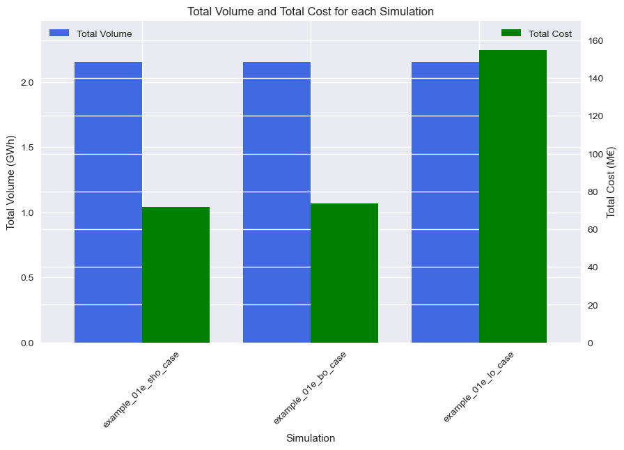
In the first plot, the total traded volume and the total costs for generation are displayed. We can see, that the total volume does not change, because we have an inflexible demand, which is always met. The total costs show significant differences only when linked orders are introduced.
Because the bidding prices are formed using the same rules, it was expected, that the introduction of new order types with additional restrictions increase prices and costs, as shown in this plot for linked orders.
Now we create the second plot, showing the accepted volumes for the different simulations for the hard coal unit.
[19]:
# second plot for the accepted volume of the coal unit
sql = """
SELECT
  start_time as "time",
  sum(accepted_volume) AS "accepted_volume",
  unit_id,
  simulation,
  bid_type
FROM market_orders
WHERE
  start_time between '2020-01-22' And '2020-01-25' AND
  unit_id = 'coal_unit' AND
  simulation in ('example_01e_sho_case', 'example_01e_bo_case', 'example_01e_lo_case')
GROUP BY 1, unit_id, simulation, bid_type
ORDER BY 1
"""

df = pd.read_sql(sql, engine, index_col="time")

df=df.sort_values(by='simulation',
                        key=lambda x: x.map({'example_01e_sho_case': 1,
                                             'example_01e_bo_case': 2,
                                             'example_01e_lo_case': 3})
                                            )

fig, ax = plt.subplots(3,1, figsize=(10,10))

#plot the sum of accepted volume for each simulation over time
for i, sim in enumerate(df.simulation.unique()):
    data=df[df.simulation == sim].sort_index()
    #set index to datetime
    data.index = pd.to_datetime(data.index)
    #sum over bid_types
    data=data["accepted_volume"].groupby([data.index]).sum()
    #reset index and fill empty data points with zero
    time_index = pd.date_range(start=min(df.index), end=max(df.index), freq='1h')
    data=data.reindex(time_index, fill_value=0.0)
    data.plot(ax=ax[i], label=sim, color='royalblue', linestyle='-')
    ax[i].set_title(sim)
    ax[i].set_ylabel("Accepted Power (MW)")
    if i < 2:
        ax[i].set_xlabel("")
        ax[i].set_xticklabels([])
    ax[i].legend(['hard coal unit'], loc='upper right')

    # add horizontal corridor for min and max power
    ax[i].fill_between(data.index, 385.5, 950, color='lightgreen', alpha=0.5)
    ax[i].fill_between(data.index, 0, 385.5,
                       where=(data > 0) & (data < 385.5),
                      color='lightcoral', alpha=0.5
                      )

#set the xticks for the last subplot
ax[2].set_xlabel("Time")

savefig("accepted-power.png")
plt.show()
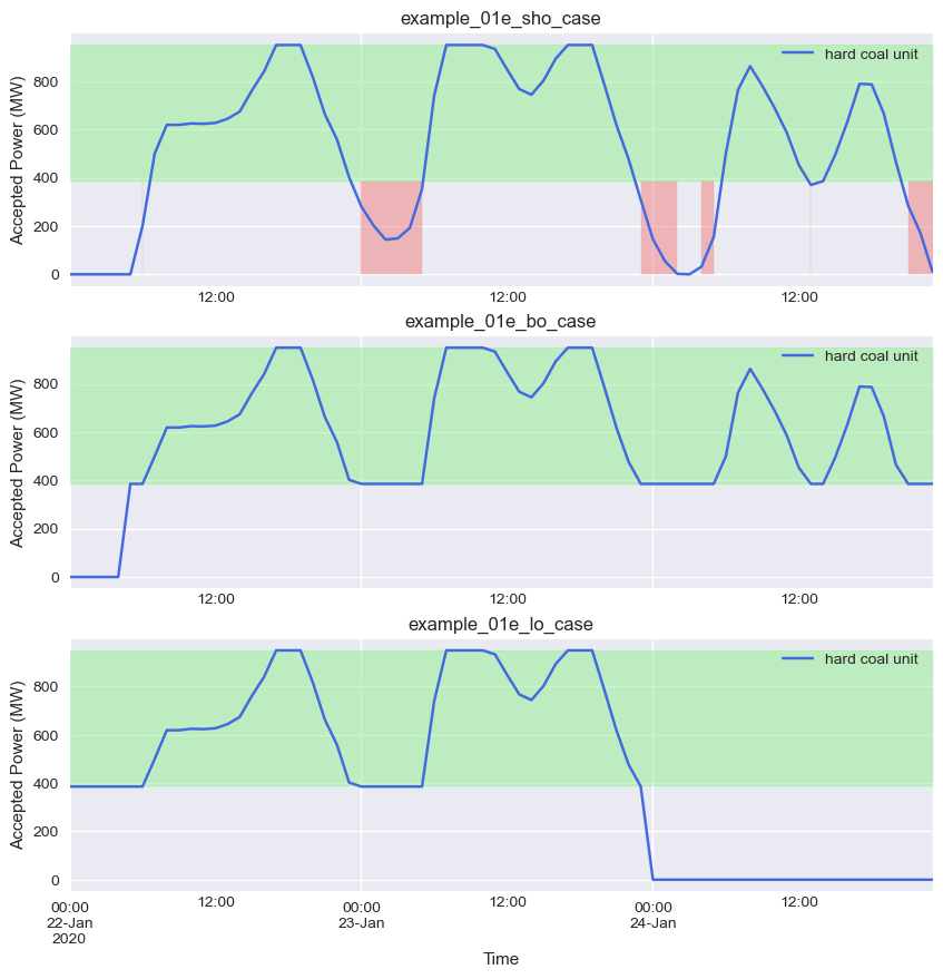
Here, you can see that the accepted power of the hard coal unit depends on the order type. The unit has a minimum power output of 385.8 MW and a maximum of 950 MW. The plot shows that in the SHO-case the minimum power restriction is not always respected. But also in the BO-case the accepted volume can be between zero and the minimum power output, because it is possible to accept the flexible single hourly bid without accepting the block bid. With the linked orders all technical restrictions can be represented in the strategy. Therefore, the dispatch of the unit can precisely follow the market outcome, but the sum of the accepted volume is slightly lower.
This brings us to the end of this short tutorial on advanced orders.