Note
You can download this example as a Jupyter notebook or try it out directly in Google Colab.
3. Implementation of a Demand Side Unit and Bidding Strategy#
This tutorial provides a step-by-step guide for implementing a custom Demand Side Unit with a Rule-Based Bidding Strategy in the ASSUME framework. By the end of this guide, you will be familiar with the process of creating and integrating a Demand Side Agent within the electricity market simulation environment provided by ASSUME.
We will cover the following topics:
Essential concepts and terminology in electricity market modeling
Setting up the ASSUME framework
Developing a new Demand Side Unit
Formulating a rule-based bidding strategy
Integrating the new unit and strategy into the ASSUME simulation
1. Introduction to Unit Agents and Bidding Strategy#
The ASSUME framework is a versatile tool for simulating electricity markets, allowing researchers and industry professionals to analyze market dynamics and strategies.
A Unit in ASSUME refers to an entity that participates in the market, either buying or selling electricity. Each unit operates based on a Bidding Strategy, which dictates its market behavior. For Demand Side Management (DSM) Units, this includes adjusting electricity demand in response to market conditions.
In this tutorial, we will create a DSM Unit that represents an Electrolyser, capable of varying its demand to optimize for energy prices.
Understanding Demand Side Management (DSM)
Before we start coding, it’s essential to understand what DSM is and why it’s important in electricity market modeling. DSM allows for the dynamic adjustment of electricity demand, contributing to balanced grid operations.
Understanding the Model
The image below illustrates the concept of a simple Electrolyser unit model:
[38]:
# this cell is used to display the image in the notebook when using collab
# or running the notebook locally

from IPython.display import Image, display
import os

image_path = "assume/docs/source/img/Electrolyzer.png"
alt_image_path = "../../docs/source/img/Electrolyzer.png"

if os.path.exists(image_path):
    display(Image(image_path))
elif os.path.exists(alt_image_path):
    display(Image(alt_image_path))
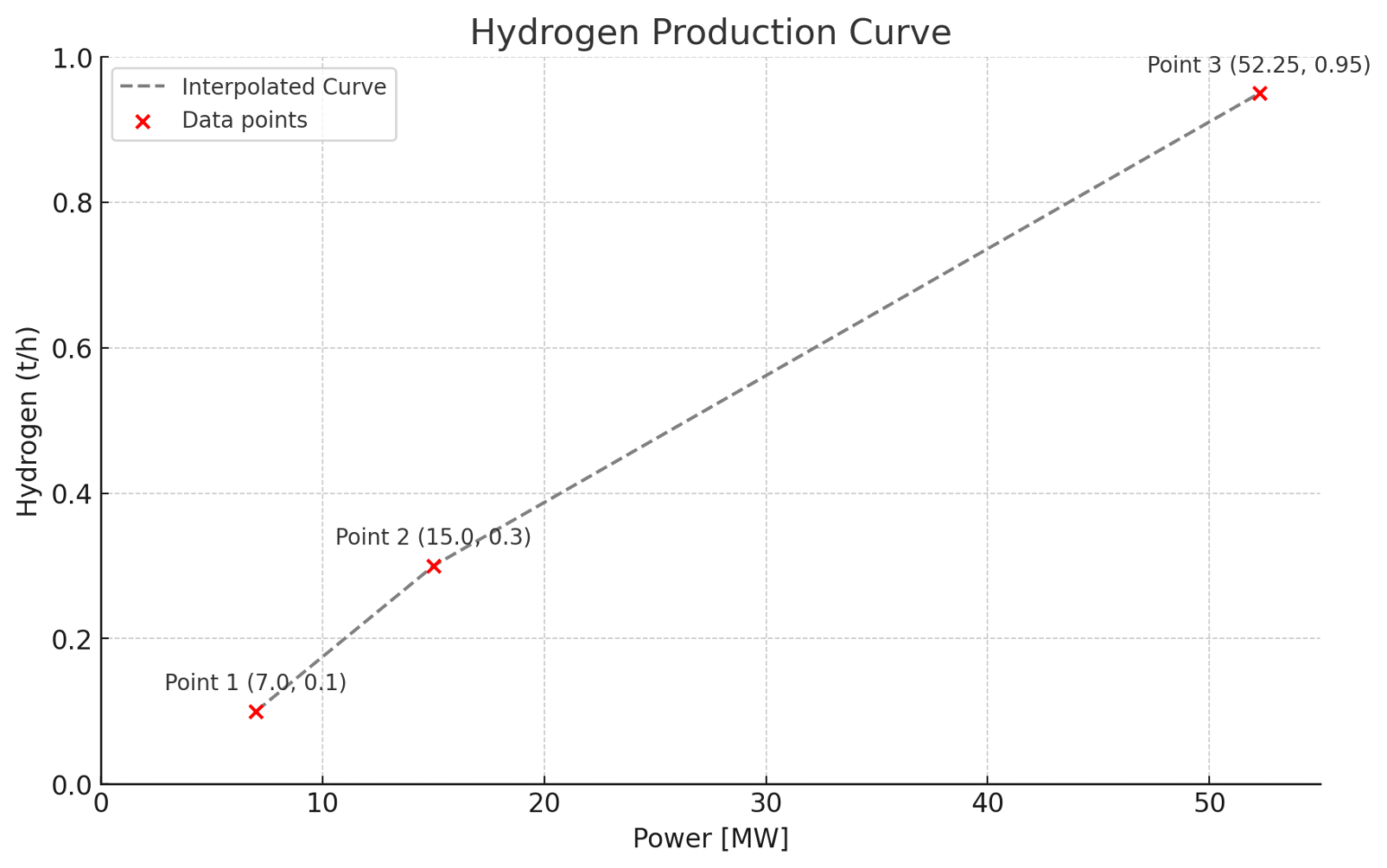
The image provides a visual representation of how dynamic efficiency varies based on different factors:
X-Axis: Represents the varying power input to the Electrolyser unit.
Y-Axis: Indicates the efficiency levels that correspond to different power inputs.
Curve: Shows that the efficiency is not constant and varies depending on the current power input to the unit.
Significance of this model
Understanding this model is crucial for several reasons:
Adaptability: The curve suggests that the unit can operate at different efficiency levels, allowing it to adapt to market conditions.
Optimization: Knowing the efficiency levels at various power inputs allows the unit to operate at an optimal point, which is especially crucial in Demand Side Management (DSM) strategies.
Complexity: The non-linear nature of the curve indicates that simple linear models may not be sufficient for capturing the unit’s behavior, highlighting the need for a more complex model.
By understanding this model, you’ll gain valuable insights into how to calculate and utilize dynamic efficiency in the Electrolyser unit, a crucial aspect of DSM in the ASSUME framework.
2. Setting Up ASSUME#
Before we create our custom unit, let’s set up the ASSUME framework. We’ll install the ASSUME core package and clone the repository containing predefined scenarios.
[ ]:
!pip install assume-framework
!git clone https://github.com/assume-framework/assume.git
Note that Google Colab does not support Docker functionalities, so features dependent on Docker will not be available here.
3. Developing a New Demand Side Unit#
We will now develop a new unit that models an Electrolyser. This unit will be capable of adjusting its electricity consumption based on the market conditions, showcasing DSM capabilities.
3.1 Initializing Core Attributes#
We’ll start by defining the core attributes of our Electrolyser class, such as its power capacity and operational parameters.
ID: A unique identifier for the unit.
Technology: The type of technology used, which in this case is electrolysis for hydrogen production.
Unit Operator: The entity responsible for operating the unit.
Bidding Strategies: The strategies used by the unit for bidding in the electricity market.
Max Power and Min Power: The maximum and minimum electrical power that the unit can handle.
Max Hydrogen and Min Hydrogen: The maximum and minimum hydrogen production levels.
Fixed Cost: The fixed operational cost for the unit.
[17]:
# Initialize the Electrolyser class with core attributes

import pandas as pd
from assume.common.base import SupportsMinMax, BaseStrategy
from assume.common.market_objects import MarketConfig, Order, Orderbook, Product


class Electrolyser(SupportsMinMax):
    def __init__(
        self,
        id: str,
        technology: str,
        index: pd.DatetimeIndex,
        unit_operator: str,
        bidding_strategies: str,
        max_power: float,
        min_power: float,
        max_hydrogen: float,
        min_hydrogen: float,
        additional_cost: float,
        **kwargs,
    ):
        super().__init__(
            id=id,
            unit_operator=unit_operator,
            technology=technology,
            bidding_strategies=bidding_strategies,
            index=index,
            **kwargs,
        )

        self.min_hydrogen = min_hydrogen
        self.max_hydrogen = max_hydrogen

        self.max_power = max_power
        self.min_power = min_power
        self.additional_cost = additional_cost

        self.conversion_factors = self.get_conversion_factors()

    # this function is a must be part of any unit class
    # as it controls how the unit is dispatched after market clearings
    # and is executed after each market clearing
    def execute_current_dispatch(
        self,
        start: pd.Timestamp,
        end: pd.Timestamp,
    ):
        end_excl = end - self.index.freq

        # Calculate mean power for this time period
        avg_power = abs(self.outputs["energy"].loc[start:end_excl]).mean()

        # Decide which efficiency point to use
        if avg_power < self.min_power:
            self.outputs["energy"].loc[start:end_excl] = 0
            self.outputs["hydrogen"].loc[start:end_excl] = 0
        else:
            if avg_power <= 0.35 * self.max_power:
                dynamic_conversion_factor = self.conversion_factors[0]
            else:
                dynamic_conversion_factor = self.conversion_factors[1]

            self.outputs["energy"].loc[start:end_excl] = avg_power
            self.outputs["hydrogen"].loc[start:end_excl] = (
                avg_power / dynamic_conversion_factor
            )

        return self.outputs["energy"].loc[start:end_excl]

    # this function is a must be part of each unit class
    # as it dictates which parameters of the unit we would like to save to the databse
    # or csv files
    def as_dict(self) -> dict:
        unit_dict = super().as_dict()
        unit_dict.update(
            {
                "max_power": self.max_power,
                "min_power": self.min_power,
                "min_hydrogen": self.min_hydrogen,
                "max_hydrogen": self.max_hydrogen,
                "unit_type": "electrolyzer",
            }
        )
        return unit_dict
Why Are These Attributes Important?
Understanding these attributes is crucial for the following reasons:
They define the range of actions the Electrolyser unit can perform in the electricity market.
They are used to calculate dynamic efficiency and power input, as we’ll see in the later sections.
They can be crucial for implementing demand-side management strategies, where the unit adjusts its operations based on market signals.
3.2 Power Calculation Function#
Next, we’ll implement a function to calculate the power input for the Electrolyser based on its demand profile. This function calculates the amount of electrical power that should be supplied to the unit, taking into consideration several attributes like maximum capacity, demand profile, and dynamic efficiency.
This function is integral for: - Optimizing Resource Utilization: Ensuring that the Electrolyser operates within its optimal efficiency range. - Demand-Side Management (DSM): Allowing the unit to adapt its power consumption in response to market signals and constraints, thereby contributing to grid stability.
Key Parameters Involved - Maximum and Minimum Capacity: The upper and lower bounds for power input to the Electrolyser. - Demand Profile: The expected hydrogen production rates, which influence the power requirements. - Dynamic Efficiency: The efficiency of converting power to hydrogen at different levels of power input, as discussed in the previous section.
[18]:
# we define the class again and inherit from the initial class just to add the additional method to the original class
# this is a workaround to have different methods of the class in different cells
# which is good for the purpose of this tutorial
# however, you should have all functions in a single class when using this example in .py files


class Electrolyser(Electrolyser):
    def calculate_min_max_power(
        self,
        start: pd.Timestamp,
        end: pd.Timestamp,
        hydrogen_demand=0,
    ):
        # check if hydrogen_demand is within min and max hydrogen production
        # and adjust accordingly
        if hydrogen_demand < self.min_hydrogen:
            hydrogen_production = self.min_hydrogen

        elif hydrogen_demand > self.max_hydrogen:
            hydrogen_production = self.max_hydrogen

        else:
            hydrogen_production = hydrogen_demand

        # get dynamic conversion factor
        dynamic_conversion_factor = self.get_dynamic_conversion_factor(
            hydrogen_production
        )
        power = hydrogen_production * dynamic_conversion_factor

        return power, hydrogen_production
3.3 Developing Advanced Attributes#
We will enhance our Electrolyser class by adding advanced attributes like dynamic efficiency, which varies with power input.
Dynamic efficiency refers to the Electrolyser unit’s ability to convert electrical power into hydrogen gas at varying rates of efficiency, depending on its current power input. This attribute is crucial for the following reasons:
It allows the unit to adapt to fluctuating market conditions, optimizing its operation for price signals.
It provides a quantitative measure for decision-making, particularly in DSM where the unit may need to adjust its demand profile.
Key Parameters Involved
Average Power: The mean power consumed during a specific time period.
Conversion Factors: These are factors used to convert the average power into hydrogen production, and they can vary based on the power level.
[19]:
# we define the class again and inherit from the initial class just to add the additional method to the original class
# this is a workaround to have different methods of the class in different cells
# which is good for the purpose of this tutorial
# however, you should have all functions in a single class when using this example in .py files


class Electrolyser(Electrolyser):
    def get_dynamic_conversion_factor(self, hydrogen_demand=None):
        # Adjust efficiency based on power
        if hydrogen_demand <= 0.35 * self.max_hydrogen:
            return self.conversion_factors[0]
        else:
            return self.conversion_factors[1]

    def get_conversion_factors(self):
        # Calculate the conversion factor for the two efficiency points
        conversion_point_1 = (0.3 * self.max_power) / (
            0.35 * self.max_hydrogen
        )  # MWh / Tonne
        conversion_point_2 = self.max_power / self.max_hydrogen  # MWh / Tonne

        return [conversion_point_1, conversion_point_2]
4. Rule-Based Bidding Strategy#
Now, we’ll define a rule-based bidding strategy for our Electrolyser unit. This strategy will use market information to place bids.
Key components of a Rule-Based Bidding Strategy 1. Product Type: This sets the stage for the kind of products (e.g., energy, ancillary services) that the unit will bid for in the electricity market. 2. Bid Volume: The quantity of the product that the unit offers in its bid. 3. Marginal Revenue: Used to determine the price at which the unit should make its bid. This involves calculating the unit’s incremental revenue for additional units of electricity sold or consumed.
The NaiveStrategyElectrolyser class inherits from the BaseStrategy class and implements the calculate_bids method, which is responsible for formulating the market bids:
calculate_bids method takes several arguments, including the unit to be dispatched (unit), the market configuration (market_config), and a list of products (product_tuples). It returns an Orderbook containing the bids.
In this case, we use Marginal Revenue to determine the price at which the unit should make its bid. The equation used in the code is as follows:
where: - Hydrogen Price: The price of hydrogen at the specific time frame, fetched from the unit’s forecaster. - Fixed Cost: The constant cost associated with the unit, not varying with the amount of power or hydrogen produced. - Hydrogen Production: The amount of hydrogen produced during the given time frame, calculated based on the hydrogen demand. - Power: The electrical power consumed by the Electrolyser unit to produce the given amount of hydrogen.
This mathematical equation provides just a mere example for understanding and implementing an effective rule-based bidding strategy for the Electrolyser unit.
[20]:
class NaiveStrategyElectrolyser(BaseStrategy):
    def calculate_bids(
        self,
        unit: SupportsMinMax,
        market_config: MarketConfig,
        product_tuples: list[Product],
        **kwargs,
    ) -> Orderbook:
        """
        Takes information from a unit that the unit operator manages and
        defines how it is dispatched to the market
        """
        start = product_tuples[0][0]  # start time of the first product
        bids = []

        # iterate over all products
        # to create a bid for each product
        # in this case it would be 24 bids for each hour of the day-ahead market
        for product in product_tuples:
            """
            for each product, calculate the marginal revenue of the unit at the start time of the product
            and the volume of the product. Dispatch the order to the market.
            """

            # get the start and end time of the product
            # for example 1 AM to 2 AM
            start = product[0]
            end = product[1]

            # Get hydrogen demand and price for the product start time
            # in this case for the start hour of the product
            hydrogen_demand = unit.forecaster[f"{unit.id}_h2demand"].loc[start]
            hydrogen_price = unit.forecaster[f"{unit.id}_h2price"].loc[start]

            # Calculate the required power and the actual possible hydrogen production
            # given the hydrogen demand
            power, hydrogen_production = unit.calculate_min_max_power(
                start=start,
                end=end,
                hydrogen_demand=hydrogen_demand,
            )

            # Calculate the marginal revenue of producing hydrogen
            # as described in the equation above
            marginal_revenue = (
                (hydrogen_price - unit.additional_cost) * hydrogen_production / power
            )

            # set the bid price to the marginal revenue
            bid_price = marginal_revenue

            # formulate the order
            # start, end, price, and volume are required
            order: Order = {
                "start_time": product[0],
                "end_time": product[1],
                "price": bid_price,
                "volume": -power,
            }

            # append the order to the list of bids
            bids.append(order)

        bids = self.remove_empty_bids(bids)

        return bids
5. Integrating the New Unit and Strategy into ASSUME#
Finally, we’ll integrate our new unit and bidding strategy into the ASSUME simulation environment.
[23]:
# import packages
import logging
import os
from datetime import datetime, timedelta

import pandas as pd
from dateutil import rrule as rr

from assume import World
from assume.common.forecasts import CsvForecaster, NaiveForecast
from assume.common.market_objects import MarketConfig, MarketProduct

logger = logging.getLogger(__name__)

# define output path
csv_path = "./outputs"
os.makedirs("./local_db", exist_ok=True)

# create world isntance
world = World(export_csv_path=csv_path)

# add new unit type to world
world.unit_types["electrolyser"] = Electrolyser
# add new bidding strategy to world
world.bidding_strategies["electrolyser_naive"] = NaiveStrategyElectrolyser


async def init():
    # define simulation period and ID
    start = datetime(2019, 1, 1)
    end = datetime(2019, 1, 30)
    index = pd.date_range(
        start=start,
        end=end + timedelta(hours=24),
        freq="H",
    )
    sim_id = "electrolyser_demo"

    # run world setup to create simulation and different roles
    # this creates the clock and the outputs role
    await world.setup(
        start=start,
        end=end,
        save_frequency_hours=None,
        simulation_id=sim_id,
        index=index,
    )

    # define market design and add it to a market
    marketdesign = [
        MarketConfig(
            market_id="EOM",
            opening_hours=rr.rrule(rr.HOURLY, interval=1, dtstart=start, until=end),
            opening_duration=timedelta(hours=1),
            market_mechanism="pay_as_clear",
            market_products=[
                MarketProduct(
                    duration=timedelta(hours=1),
                    count=1,
                    first_delivery=timedelta(hours=1),
                )
            ],
        )
    ]

    mo_id = "market_operator"
    world.add_market_operator(id=mo_id)
    for market_config in marketdesign:
        world.add_market(
            market_operator_id=mo_id,
            market_config=market_config,
        )

    # add unit operator
    world.add_unit_operator(id="power_plant_operator")

    # define a simple forecaster
    simple_forecaster = NaiveForecast(index, availability=1, fuel_price=0, co2_price=50)

    # add a unit to the world
    world.add_unit(
        id="power_plant_01",
        unit_type="power_plant",
        unit_operator_id="power_plant_operator",
        unit_params={
            "min_power": 0,
            "max_power": 100,
            "bidding_strategies": {"energy": "naive_eom"},
            "additional_cost": 5,
            "technology": "wind turbine",
        },
        forecaster=simple_forecaster,
    )

    # repeat for demand unit
    world.add_unit_operator("demand_operator")
    world.add_unit(
        id="demand_unit_1",
        unit_type="demand",
        unit_operator_id="demand_operator",
        unit_params={
            "min_power": 0,
            "max_power": 1000,
            "bidding_strategies": {"energy": "naive_eom"},
            "technology": "demand",
        },
        forecaster=NaiveForecast(index, demand=50),
    )

    # load forecasts for hydrogen demand and hydrogen price
    hydrogen_forecasts = pd.read_csv(
        "assume/examples/inputs/example_03a/forecasts_df.csv",
        index_col=0,
        parse_dates=True,
    )

    # add the electrolyser unit to the world
    world.add_unit_operator(id="electrolyser_operator")
    hydrogen_plant_forecaster = CsvForecaster(index=index)
    hydrogen_plant_forecaster.set_forecast(data=hydrogen_forecasts)

    world.add_unit(
        id="elektrolyser_01",
        unit_type="electrolyser",
        unit_operator_id="electrolyser_operator",
        unit_params={
            "min_power": 7,
            "max_power": 52.25,
            "min_hydrogen": 0.15,
            "max_hydrogen": 0.95,
            "bidding_strategies": {"energy": "electrolyser_naive"},
            "technology": "electrolyser",
            "additional_cost": 10,
        },
        forecaster=hydrogen_plant_forecaster,
    )


# run the simulation
world.loop.run_until_complete(init())
world.run()
electrolyser_demo 2019-01-30 00:00:00: : 2505601.0it [00:05, 463038.19it/s]
The above code block is more in line with Tutorial 1, where we manually defined the simulation and executed it. It shows all inner working and serves better understanding.
For more practical applications you should use the construct from Tutorial 2 to have an automated loading and execution of the scenario, where all parameters are defined in a configuration file, as in the following code block.
For more details on the configuration and input files structure check out the example_03a folder in examples folder.
[25]:
# import the main World class and the load_scenario_folder functions from assume
from assume import World
from assume.scenario.loader_csv import load_scenario_folder

# Set up logging
log = logging.getLogger(__name__)

# Define paths for input and output data
csv_path = "outputs"

# Create directories if they don't exist
os.makedirs("local_db", exist_ok=True)

# make sure that you have a database server up and running - preferabely in docker
# DB_URI = "postgresql://assume:assume@localhost:5432/assume"
# but you can use a file-based sqlite database too:
data_format = "local_db"  # "local_db" or "timescale"

if data_format == "local_db":
    db_uri = f"sqlite:///./local_db/assume_db_example_03.db"
elif data_format == "timescale":
    db_uri = "postgresql://assume:assume@localhost:5432/assume"

# create world
world = World(database_uri=db_uri, export_csv_path=csv_path)

# load scenario by providing the world instance
# the path to the inputs folder and the scenario name (subfolder in inputs)
# and the study case name (which config to use for the simulation)
load_scenario_folder(
    world,
    inputs_path="assume/examples/inputs",
    scenario="example_03a",
    study_case="base",
)

# run the simulation
world.run()
example_03a_base 2019-01-30 00:00:00: : 2505601.0it [00:03, 629000.05it/s]
This concludes our tutorial. By following these steps, you have successfully created a Demand Side Unit with a Rule-Based Bidding Strategy and integrated it into the ASSUME framework.